Getting started

Run in Lumicron

Lumicron includes Python 3.12 and its matching lumicron package. Create or open a project, create a Python file in Script, and use Run. No separate Python installation is required for the bundled runtime. For standalone development, use an environment containing this same API and its dependencies; an unrelated installed package may expose a different API.

The examples use the bundled educational elyon_demo PDK. It demonstrates the API and is not a fabrication-qualified foundry process. Use your project’s installed PDK for real designs.

Hello, Lumicron

The smallest meaningful script: one cell, one rectangle, one GDS file. The explicit export in these standalone examples also works from the app.

"""Hello, Lumicron — your first cell.

The smallest meaningful Lumicron script: one cell, one rectangle, one
GDS file. If this runs, your install is healthy.
"""
import lumicron as lm

METAL = lm.LayerSpec(layer=4, datatype=0)


@lm.pcell
def HelloLumicron():
    c = lm.CELL("HelloLumicron")
    pad = lm.Rectangle(x_dim=80, y_dim=80, layer=METAL)
    c.add(pad)
    c.Place(pad).at((0, 0))
    return c


if __name__ == "__main__":
    HelloLumicron().to_gds("hello_lumicron.gds")

Run it:

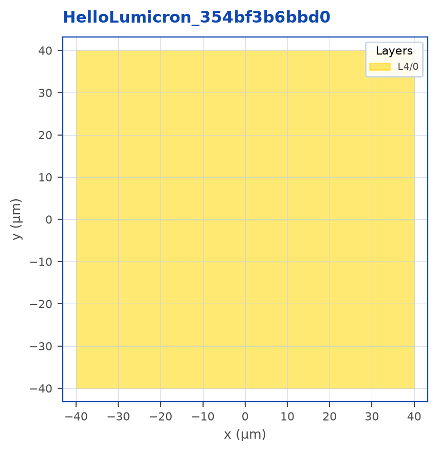
python 01_hello_world.py

If 01_hello_world.gds lands in your working directory, you’re set up. Open it in any GDS viewer (KLayout, the Lumicron Mac app, your foundry’s tool) and you’ll see an 80 × 80 µm metal pad at the origin.

A more interesting first chip

Real layouts have multiple shapes on multiple layers. This one adds a die outline, a ring resonator, and two metal pads.

"""A frame, a ring, two pads — the canonical first chip.

Three concepts in one file:
    1. Multiple shapes on different layers.
    2. Placement at explicit coordinates.
    3. Hierarchy: this cell is reusable later.
"""
import lumicron as lm

OUTLINE = lm.LayerSpec(layer=63, datatype=0)
METAL = lm.LayerSpec(layer=4, datatype=0)
SILICON = lm.LayerSpec(layer=9, datatype=0)


@lm.pcell
def FirstChip():
    c = lm.CELL("FirstChip")

    # Die outline: 2 mm × 1 mm. Place anchored at the south-west corner
    # so the chip occupies (0, 0) → (2000, 1000).
    frame = lm.Rectangle(x_dim=2000, y_dim=1000, layer=OUTLINE)
    c.add(frame)
    c.Place(frame).using("SW").at((0, 0))

    # A silicon ring resonator, off-center.
    ring = lm.Ring(outer_radius=50, width=4, layer=SILICON)
    c.add(ring)
    c.Place(ring).at((600, 500))

    # Two metal pads. We capture each handle from c.add() so each call
    # to Place() targets a distinct instance — re-using the same `pad`
    # spec without capturing would just move the most-recent placement.
    pad = lm.Rectangle(x_dim=80, y_dim=80, layer=METAL)
    pad_top = c.add(pad)
    pad_bot = c.add(pad)
    c.Place(pad_top).at((1700, 750))
    c.Place(pad_bot).at((1700, 250))
    return c


if __name__ == "__main__":
    FirstChip().to_gds("first_chip.gds")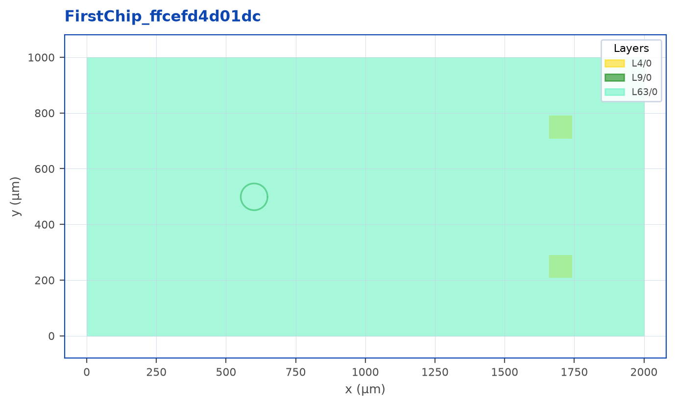

Three patterns to internalize from this example:

1. Define, add, place. Build a shape, hand it to the cell with c.add(...), then locate it with c.Place(...).at(...).
2. Capture the handle when you need multiple copies. pad_top = chip.add(pad) returns a fresh handle for that specific instance. Each chip.add(pad) creates a distinct placed object. Keep both handles to move the two placements independently.
3. .using("SW") overrides the default placement anchor. By default at((x, y)) puts the bbox center at (x, y). The frame uses using("SW") to anchor at the south-west corner instead, so the chip spans (0, 0) to (2000, 1000) rather than centering on the origin.

What you just used

The next chapter formalizes these into a vocabulary you’ll use everywhere.

Phoebe Guide and native circuit experiments

Choose Help → Start Phoebe Guide to open or resume an editable project using Lumicron Demo PDK 0.1.0 and its separate validation package. Build one MZI, simulate it, generate its physical Layout, verify it, prepare its Registry and curate a Notebook record. The Demo platform is fictional and educational, not fabrication qualified.

The short Product Tour introduces the application on first use. Replay it from Settings → Phoebe → Replay Product Tour. Open Phoebe Guide in the same Settings pane opens or resumes the separate engineering project; it never starts MZI instructions over an unrelated project. Existing project windows and unsaved work remain intact. Explicit Restart creates a fresh UUID-scoped copy. Choose a lesson from Lessons. Phoebe’s spotlight follows real controls and objects; Continue always works, even when a target or result is unavailable. Engineering completion never advances the guide or turns skipped work into verified evidence. Drag the card’s header to put Phoebe where you prefer. Previous changes guidance only. Pause leaves a small Resume Guide button; More actions offers Skip, Reference, Restart and Exit. Reopening retains the project’s guide progress. Restart creates a fresh copy and preserves the previous project. Later-lesson restarts use a labeled ordinary MZI checkpoint. Legacy LearnLumicron resources and their machine identities remain readable; they are not silently converted to Demo designs.

The working project uses normal manifests, exact locks, Schematic, public Script, Layout, Registry and Notebook files. Local bundled dependencies have content digests; a Git dependency additionally has an exact revision. Refresh Dependencies reviews changes; Keep Current preserves the lock. No public Demo remote is implied. Optional Phase 18 recipes live under Reference/examples, outside the mandatory curriculum. The guide’s short instructions link to this reference for detail.

Phoebe names the control and its location whenever she asks for an interaction. For example, </> Generate Layout in the top toolbar turns the logical circuit into editable physical Python and a Layout. A spotlight uses only a real mounted target; native title-bar controls outside its host retain clear directions with no guessed highlight. Command-K opens the real Search / Commands palette during guidance. Closing it leaves you on the same card; Continue is manual.

In Schematic, place Source and Detector from the normal IdeaKit Library and wire their terminals directly to the circuit. Select a Source or Detector and open Properties for its Basic/Advanced controls. The Source sets the wavelength sweep in micrometres, normalized amplitude and phase in degrees. One Source and multiple Detectors are supported. Detectors are non-loading observations; they create no physical device or fabricated geometry. Experiment settings remain separate from component parameters and the semantic circuit. This native workflow introduces no public Python Circuit, Source or Detector API.

Select a connection and open Properties to edit its routing target, profile, bends and propagation override. Valid picker/toggle choices commit directly; text and numbers commit on Return or focus change. Generate Layout, Run Simulation and Save first resolve the focused Inspector edit. Invalid input stays visible and blocks those actions until corrected or cancelled with Escape; there is no Apply step. Accepted edits use normal Undo/Redo. An explicit propagation override takes precedence. Otherwise an explicit route profile, or matching profiles on both canonical endpoint PORTs, supplies its declared propagation model. Different endpoint profiles require an explicit choice; width and layer alone do not determine phase.

• Specified uses positive authored interconnect target lengths and declared propagation models. Schematic drawing distances are never optical lengths.
• Realized uses qualified measurements from Generate Layout. That action executes a Lumicron-owned construction transaction against the exact PCells, validates that physical candidate, then publishes editable from_schematic Python and its Layout together. The same recorded public calls and resolved arguments drive construction and source emission. A failed candidate leaves the previous generated files intact and supplies no current measurements. No separate Measure Routes step is needed. Changed circuit inputs cannot reuse stale evidence or fall back to specified lengths. User-owned edited Python is not silently rebound to the generated circuit.

Automatic physical placement supports bounded co-facing parallel interfaces, including opposing wire draw order. It may orient/reflect components and choose spacing from authored targets. PDK bend limits and targets remain unchanged; infeasible routing still fails explicitly. This is not general feedback synthesis or fabrication qualification. To take over physical placement/routing, use the ordinary generated-script ownership workflow.

Successful native Generate Layout retains the last validated realization at each generated source path in .lumicron/realizations. Script Outline shows this historical origin separately from current Layout correspondence. Removing the managed header or editing the public calls does not erase that saved evidence. Older generated files with private binding/verification calls remain runnable; new generated files do not contain those calls. Running public source independently does not recreate the managed transaction’s semantic correspondence. It can leave the new artifact’s bindings and circuit equivalence unresolved. Lumicron never matches edited instances by their names, order or geometry. The receipt is not a substitute for an admitted current sidecar, and older projects without a receipt do not acquire guessed history.

Symbol rotation and external-port body dragging change presentation only. Use the separate port terminal to draw a wire. Existing boundary-attached experiments and legacy instrument documents remain readable; the normal Library teaches directly wired Source/Detector objects.

Each attempt captures the semantic circuit revision, exact component bindings, parameters, experiment and resolved request. Completed, failed, cancelled and interrupted attempts remain in project-owned history under .lumicron/circuit-simulation. Inspect transmission, normalized output power and phase from the selected historical run. Publish to Notebook is deliberate; automatic run history and curated Notebook evidence are separate.

The plot adapts to the Simulation tray’s available space; captured inputs and diagnostics remain under Run details. Click the plot or enter a wavelength in micrometers to select a scalar measurement. Numerical selections such as 1.31060 retain that exact wavelength. Between captured samples the displayed quantity is linearly interpolated and labeled interpolated; this does not rerun SAX or create a solver sample. Values outside the captured range are not extrapolated. With no selection, Notebook receives the complete run without an invented middle-wavelength measurement. A selected measurement is published with its trace, quantity, wavelength, value, evaluation method and captured run; subsequent selection changes do not alter that Notebook record.

The initial scope is linear optical wavelength-domain simulation using declared SAX compact models. Missing packages, absent models, unsupported PORT interfaces, invalid parameters and stale realized routes fail explicitly. Executing a supplied model does not establish its fabrication accuracy. Realized hierarchy combinations without qualified route measurements remain unavailable. Existing legacy instrument circuits retain their compatibility workflow; they are not the canonical experiment model taught here.

Code → Schematic

Use cell.to_schematic() after authoring a CELL’s explicit component graph:

import lumicron as lm
import example_oband.all as oband

cell = lm.CELL("GuidePair")
a = cell.add(oband.Guide())
b = cell.add(oband.Guide())
cell.Place(b).at((100, 0))
cell.Route(a.ports["o2"], b.ports["o1"])
a.promote({"o1": "input"})
b.promote({"o2": "output"})
created = cell.to_schematic()
print(created.path)

The result is a frozen record with path (pathlib.Path), circuit_id, name, sha256, and a tuple of diagnostics. By default a new .lumsch is created under Circuits/Generated in the working project. An optional path selects a new .lumsch destination; an existing document is never overwritten.

Default filenames use the cell name and a numeric suffix when occupied; the filename is presentation, never semantic identity. For a PCell, its declared factory name supplies the engineering label instead of the generated geometry’s parameter-hash name.

Each invocation creates a new circuit and new semantic occurrence/connection identities. Reopening the saved document retains its identities. This does not synchronize edited Python with an earlier Schematic.

Immediate eligible child instances become separate components. Reused subcells retain enterable definitions. Typed Route endpoints, paired Join endpoints and explicit promotion aliases establish connections. Raw polygons, raw GDS interiors, layout-only PCells (schematic=False) and ARRAY geometry do not become inferred components or wires; coverage diagnostics identify omitted content. Missing typed endpoints or a root PORT with no established relationship cause an explicit error. Unconnected child PORTs remain unconnected. Physical extraction and LVS are separate.

When a placed PCell’s explicit Join, Route or promotion reaches an immediate schematic=False child, that PCell remains one atomic component with its declared external PORTs. Its validated internal endpoint evidence is retained, while hidden implementation children stay hidden. Other reusable circuit definitions remain enterable. This boundary does not invent a transfer model or conceal dangling endpoints; unresolved authored evidence still fails explicitly.

Exact package bindings remain attached where available. Without such a binding, the saved interface remains inspectable but a same-named library entry is never substituted. Schematic drawing coordinates are a deterministic presentation and carry no physical placement authority. Retained targets/profile/style/bend settings remain intent; measured physical length is not invented as a target. Other routing features are not automatically converted into new Schematic capabilities.

In Lumicron Script, publication waits until the entire run succeeds. Script stays active and a Schematic created toast offers Open Schematic. The action opens that exact document; dismissing it leaves Script active. A failed run publishes no conversion and offers no success action. Headless Python writes the document when the call succeeds, returns the same result and requires no GUI.